Recently, I became very interested in neural networks. So I decided to dive into it head first. I started with the theory, then moved onto the application of that theory. The following post is me documenting the creation of a neural network for recognising handwritten digits. This is a small introductory project for learning the fundamentals and theory behind neural networks. The “hello world” of neural networks is recognising 28 x 28 handwritten digits, with training data from the MNIST dataset. So thats what this is. Unfortunately, there is not much I can do for inline code and inline latex, I haven't figured out how to get it to work how I'd like, so I'll be using screenshots of latex and code. That means you won't be able to copy code (yet).

File structure

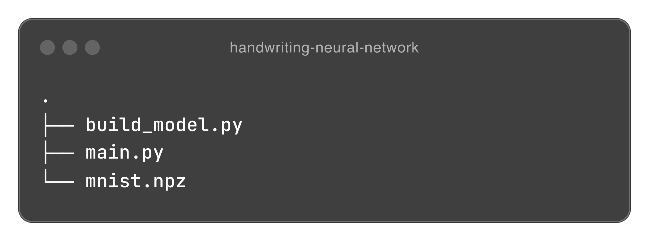
We will have one folder with two files in them. One file for defining and training our model, and the other file for loading and running our model. We’ll also download our MNIST data set online from here. Our root folder should look like this:

Building our model

We need to train our model, and to do that, we need to build it. For this task, we’ll use a multi-layer perceptron (MLP) architecture.

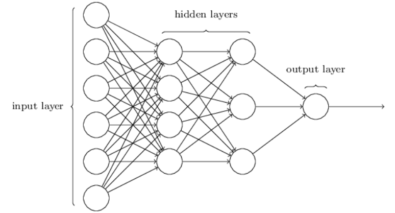
Our network will consist of:

• An input layer with 784 nodes (28x28 pixels flattened)
• Two hidden layers, each with 128 neurones
• An output layer with 10 neurones (one for each digit 0-9)

For this neural network, we’ll be using Rectified Linear Units (ReLUs) as our activation functions for our hidden layers. These help to get around the problem of vanishing gradients, which happens when gradients become extremely small during backpropagation, which makes it harder for earlier layers to learn efficiently. For a good overview, check out this article.

For our output layer, we’re going to use something called “Softmax”, which is an activation function that converts a vector of numbers into a probability distribution. It allows our network to express its confidence in each of the 10 possible digits. For example:

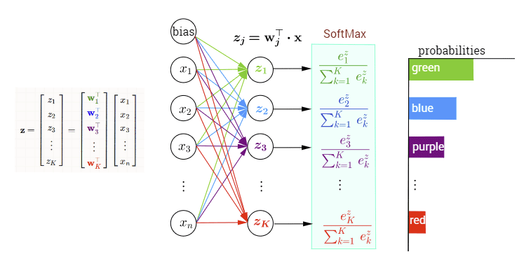
To make this make sense, we’re looking to output a possible 10 numbers:

In vector format, based on our probabilities, if we input the number 8, our distribution might look something like this:

In this case, the network determines that the probability our image is an 8 is 92%. The sum of all probabilities will always equal to 1.

Implementation

Required modules

We’ll be using a couple modules here for our application, they’re as follows:

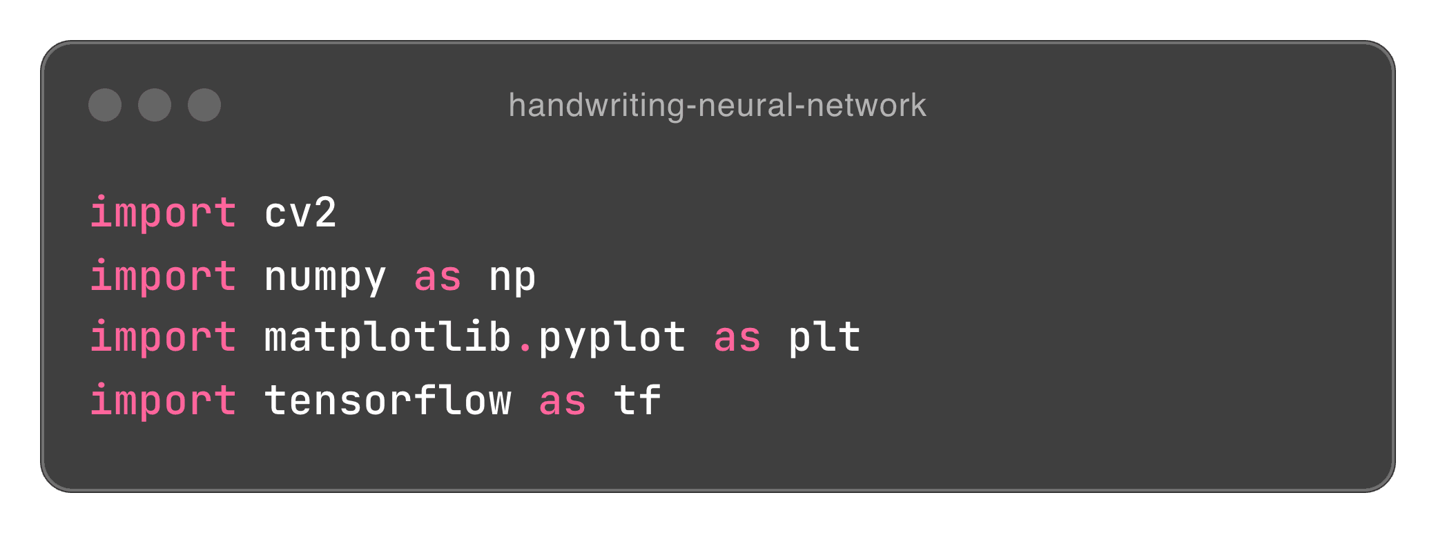
We’re using cv2 to process our images we want to identify (our actual input). We wont have to use that until our main.py file when we actually start using our trained model. We’ll go into more detail with it later on, but for know just know that its used for image processing.

Next, we’ll be using numpy, great for working with arrays an objects, something we’ll need for extracting our image data and labels, and manipulating our images.

Matplotlib is great for visualisation. Here we’re using it for plotting our input number to the screen. Again, it wont be used until the end. Really we don’t need it, but why not.

Last but not least (and the most important), we’re using Keras - a high level API built on top of Tensorflow. It will be used for creating and training our model. It provides us with a much more user friendly way to build and train models.

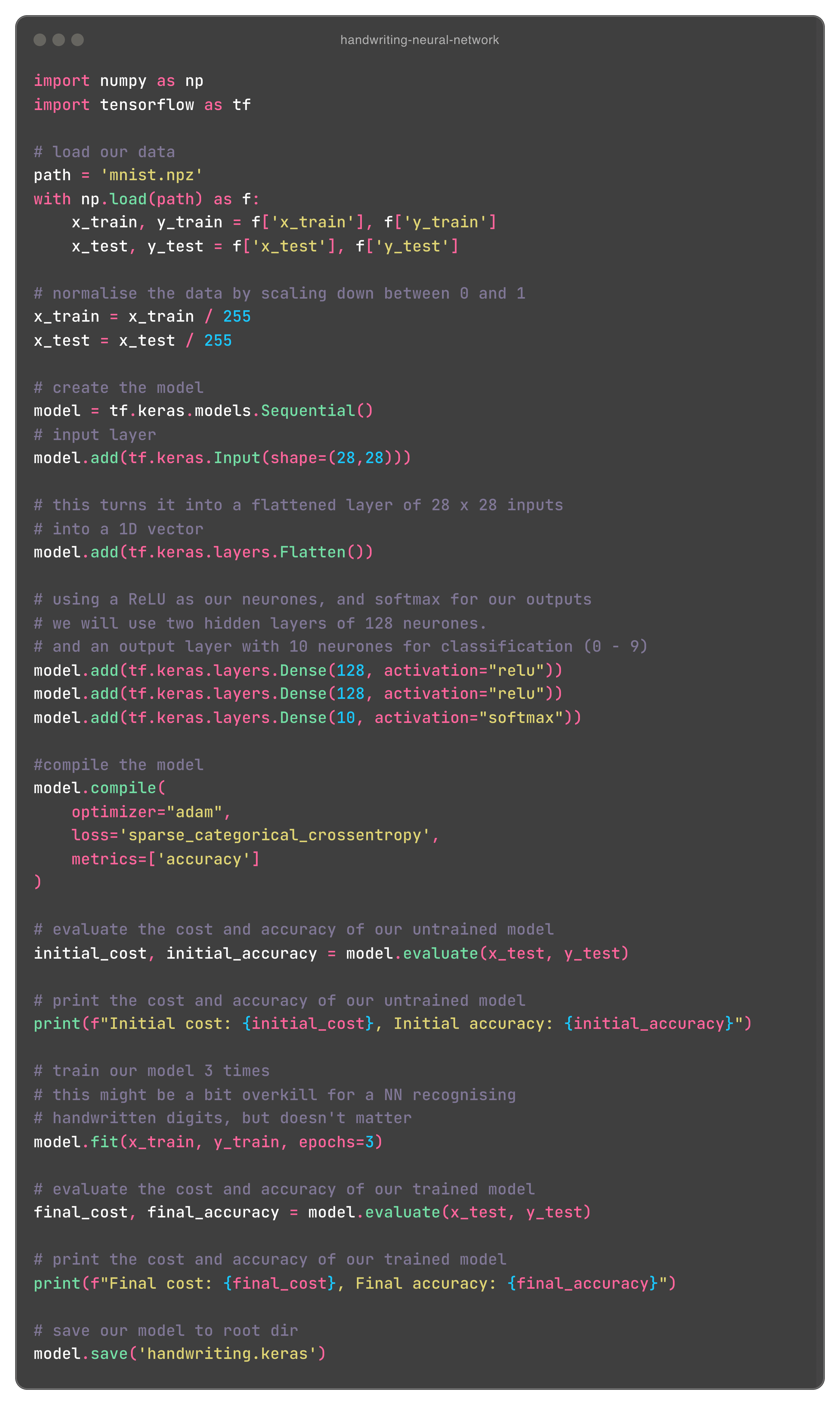
Lets get into the code, we need to load our data first from our MNIST dataset mnist.npz. We’ll define a variable named path and assign this to the location of our dataset. Technically we don’t need to do this for such a small amount of code - we’re only accessing it once - but its good to follow best practices. If we need to change the name of our file path, we can just change it in one place. Everything is in the root directory, so we don’t need to use any slashes. Now, we need to load our model using our path variable, and “unzip” our file, assigning our training data comprised of 60,000 images, and our test data comprised of 10,000 images. So far, we have something looking like this:

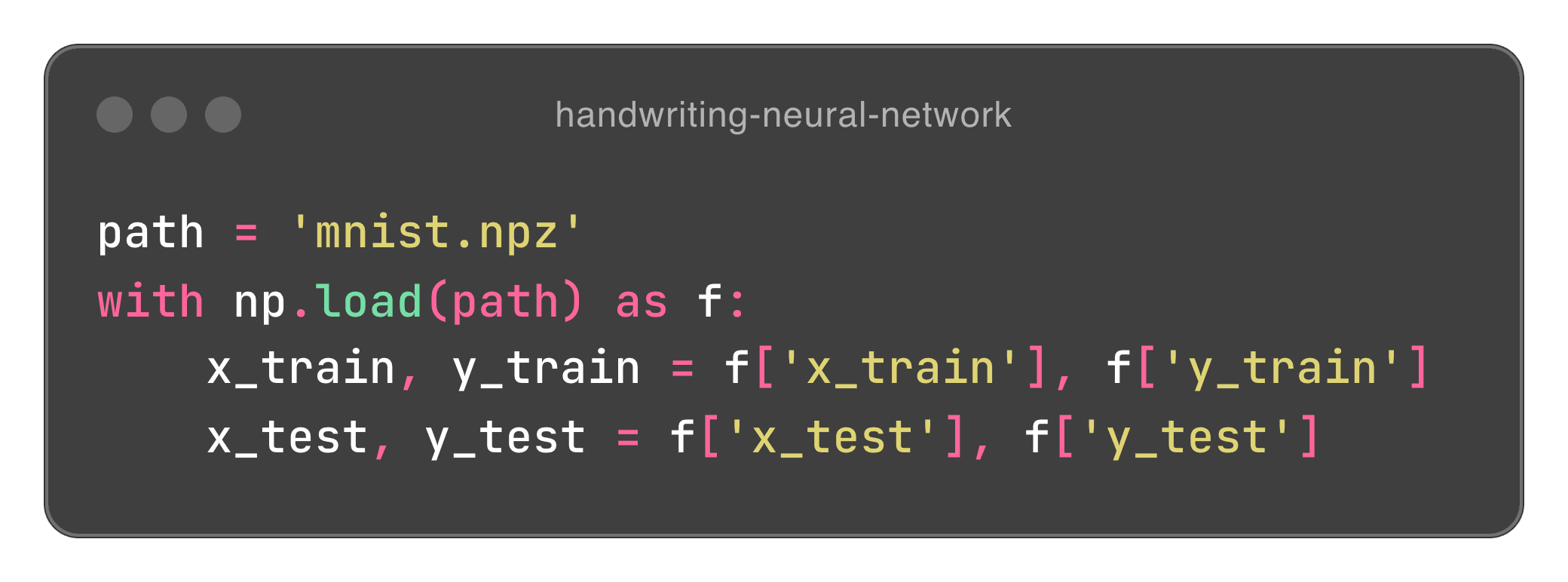
All this is saying is that, we’re going to open our file defined within our path variable, and the contents of it (a dictionary like object) will be assigned to a variable f for easy use. with ensures the file is closed after the with block. Within this block, we define four variables that are arrays. Our first line is used for defining our train data, we have x_train which is used for our actual 28 x 28 pixel images. To visualise, it’ll look something like this:

This is a greyscale image of our digits, in a 28 x 28 matrix. Each value is a pixel, which represents the “blackness” of that pixel. So, for example, 0 is completely white, yet 253 is insanely black. This basically draws our image but in an array format, which we will need for our input. Our y_train is our actual label, so let us say the above code block is of a 5, our label (since this is training data), will simply be 5. This is the exact same for our testing variables.

Normalising our data

Next we will standardise our pixel values. We can do that simply by dividing by 255:

ReLUs technically can handle larger input sizes, but its always good to standardise this. It can also help if our NN has many layers. We can see this working a little bit as the accuracy seems to improve when we do this. Our function has a (slightly) better accuracy with normalisation than without, with an accuracy of 0.9808 (98%) with normalisation, and 0.9489 (~95%) without. A small change, but for larger NN’s, it could be a bit larger.

Creating the model

Now onto the bread and butter of this project: the actual network. Here, we’re going to start by defining what type of model we want to work with. We’re going to go ahead with a sequential model. This is a linear, fastforward model which only accepts a single input and has a single output. It is a stack of layers. Heres the code block:

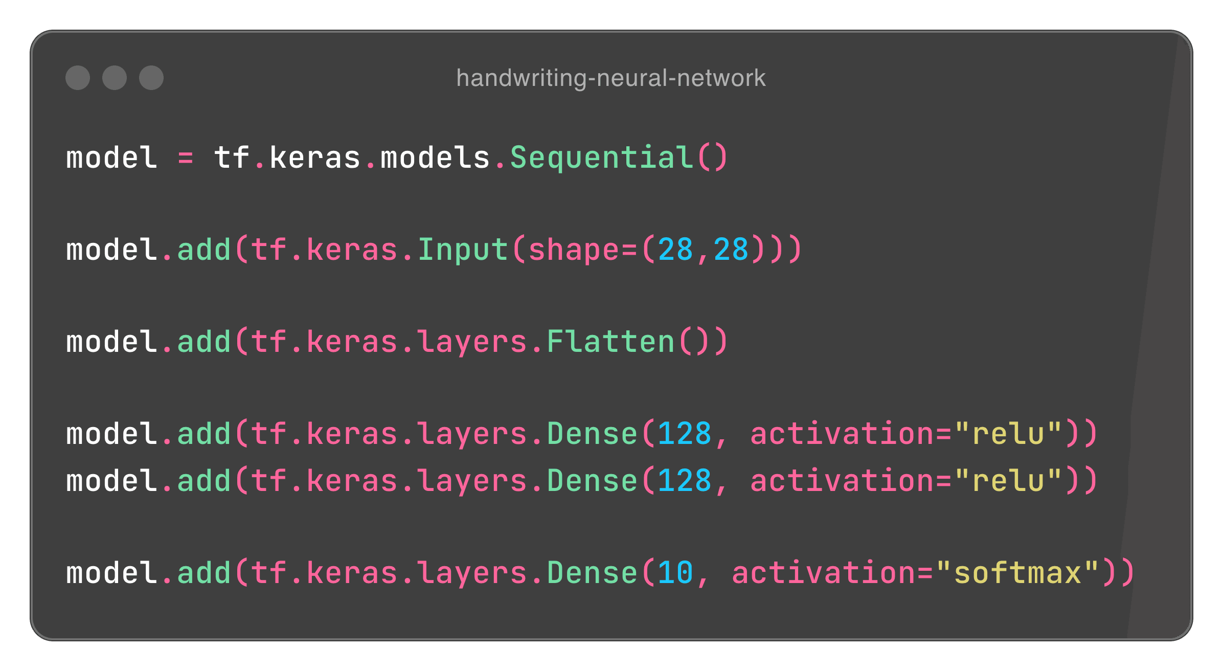
A lot of stuff going on here. Lets break it down.

First, we actually define the model we want, as explained earlier, this is a sequential model. Onto the next line, we add onto our model by defining our input with model.add(tf.keras.Input(shape=(28,28))). What this is telling us is that, we want to create an input layer with a 28 x 28 shape. This is almost what we want, but not quite. Remember, we want our input to be a 1D vector, its expecting a column vector, and so we need to flatten (transform) our input, which will look like this:

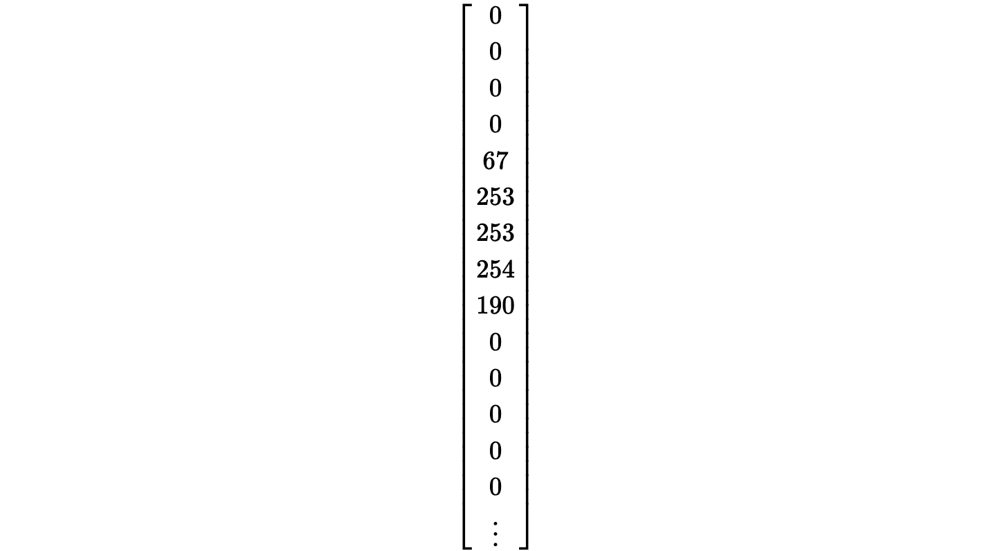
A column vector with 28 x 28 items. this is what model.add(tf.keras.layers.Flatten()) does for us.

The next two lines of code after this define which types of neurones we want for our Dense (hidden) layer. We’re saying we want 128 neurones for each hidden layer, and we want those to be ReLUs. This number is somewhat arbitrary. Really, you could use any number of neurones, and test its performance. More neurones can capture more complex patterns, but may lead to overfitting, and therefore worse accuracy. Fewer may not capture enough complexity. The right number depends on your problem.

Lastly, our output will be a layer of 10 softmax neurones. Softmax is used for multi class classification, and converts raw scores into probability distributions, talked about earlier. Heres what this looks like visually:

Next we need to compile the model. This configures how our model learns, before we actually begin training it.

Optimising with Adam

Here, we’re specifying how we plan to optimise our model. An optimiser is an algorithm that adjusts the weights and biases of our neural network to minimise our cost function during training. Earlier, we talked about stochastic gradient descent (SGD) to update our weights by moving them in the direction that reduces our cost function in batches. Adam (Adaptive Movement Estimation) is an extension of SGD. It combines ideas from two other optimisers: AdaGrad and RMSProp (we wont go into them here), and computes learning rates for our parameters. Adam keeps track of an average that exponentially decays (think of momentum) and helps adjust the learning rate individually for each parameter.

Lets say the gradient for a certain weight is large. Adam will reduce the learning rate for that weight which prevents large updates that could lead to inefficient learning. If the gradient is small, Adam will increase the learning rate, which ensures that the weights will still be updated, allowing faster but also more reliable convergence.

Cost function

We now need to specify our cost function, here, we use Sparse Categorical Cross entropy. Our problem is looking to classify each input into one of our 10 classes (0 - 9). For most multi class classification problems, Categorical Cross entropy is fine. However, with this function, it would expect a label to be encoded similar to how our input looks: as 1D vectors. For example, the digit '3' would be represented as [0, 0, 0, 1, 0, 0, 0, 0, 0, 0]. But our MNIST dataset provides our labels as integers, and SCC allows our labels to be integers, so we use that.

Accuracy

Lastly, we keep track of the accuracy of our model. It measures the proportion of correct predictions made by the model. It looks like:

We can use this to monitor how well our model performs. So during training, Keras will provide us with the loss and accuracy after each epoch (training the entire dataset once). We can see this information with the following:

We train the model with:

And save it with

When we run our file with python3 build_model.py, our terminal outputs the following:

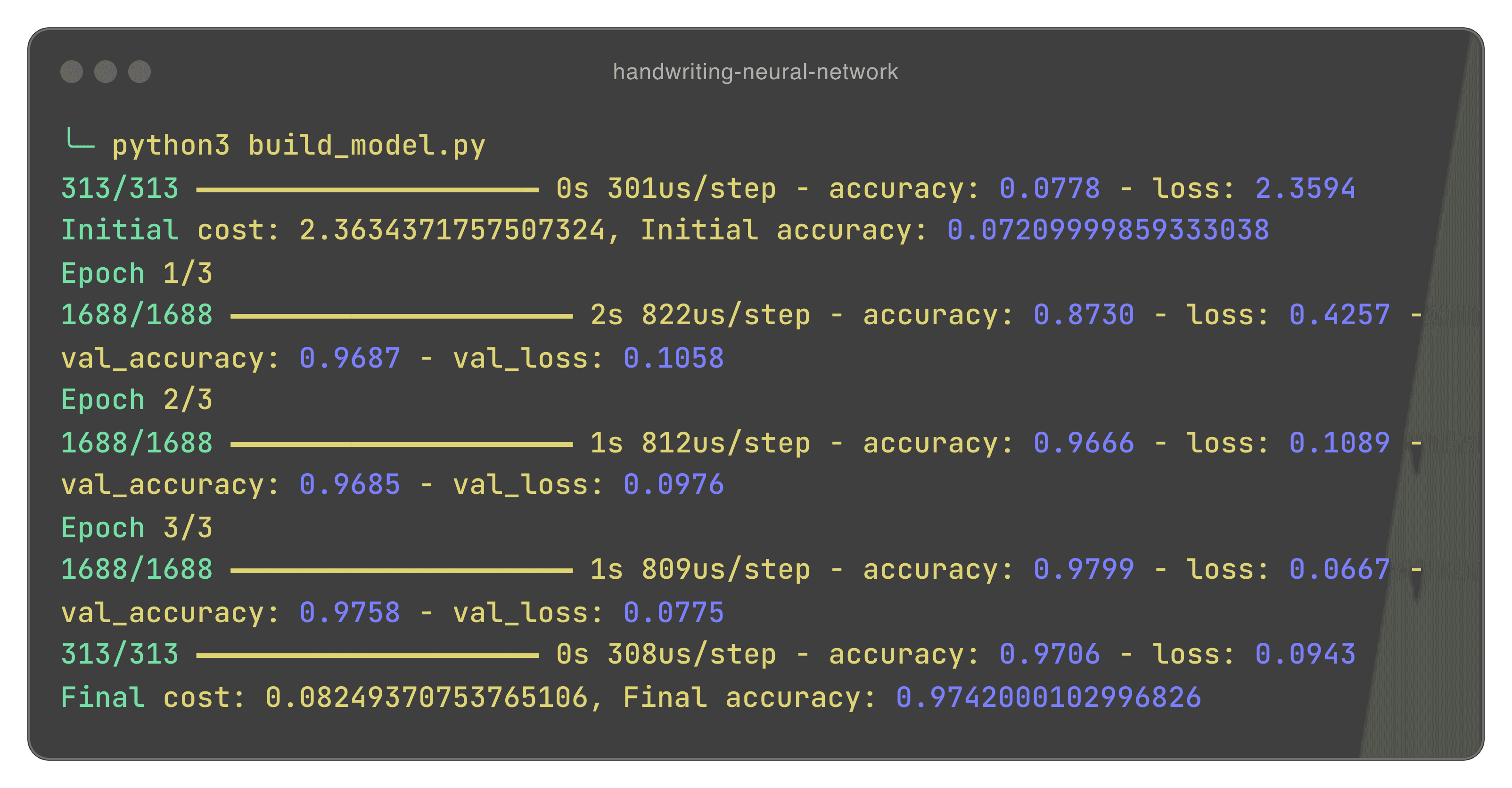
When we finally build our model, we get this output from Keras. There are a bunch of numbers, so lets dive into them.

The first thing you may notice is that, we don’t actually see 10,000 for our test, and 60,000 for our training data. Why is that? Earlier we talked about SGD and why its better. SGD divides our training and test data into mini batches, which updates our weights more frequently and allows us to refine our neural network more efficiently. We can work our how much we are dividing our test and training data by. Our first output gives us 313, which is our test data. We have 10,000 images for testing. We can work out our batch size by doing:

301us/step tells us that it takes is 301 microseconds to complete one single batch. It then tells us our initial accuracy (7%) and our initial cost (2.36). Firstly, this is not only insanely inaccurate, but our cost is far from 0. Remember, we need to get this as low as possible. The good news is that this is an analysis of our neural network before training. Immediately after, we begin training our dataset. We do it in 1688 batches of 36. Remember, we did 3 epochs, which trains our network on our dataset 3 times. All an epoch is is when we have trained our network on our entire dataset once. We do this three times, which allows us to refine our model. Not only this, but with SGD, we are able to better refine our model after each batch. After training, we see that our model has been trained very well, with a cost of 0.08, and an accuracy of around 97%.

Heres our build file:

Using our model

Now we’re going to use our model. Theres a bit of processing that needs to be done, but its very simple. Here we’ll actually use cv2 and matplotlib.

First, we load our model. Nothing to explain here. Simple stuff:

Next, we grab the image we want to identify:

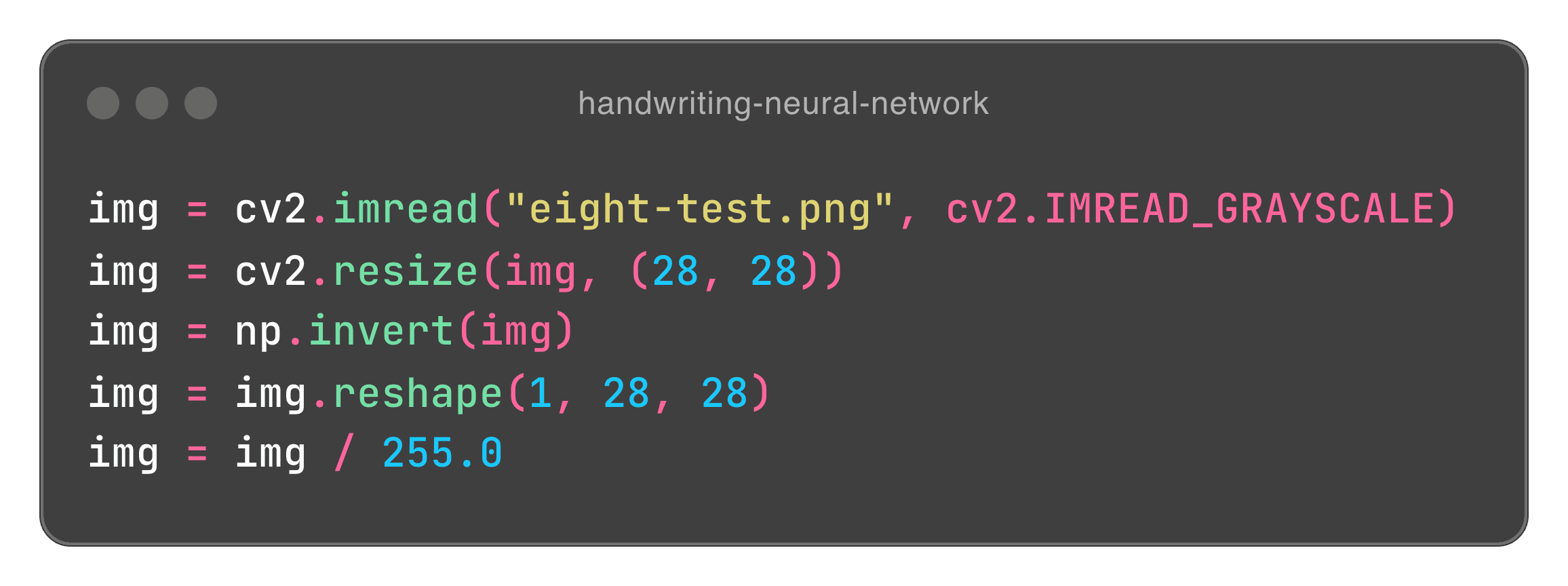
Here, we use cv2 to read our image passed in the first argument. We pass a IMREAD_GRAYSCALE parameter, because remember, we trained our model on a dataset of grayscale images. We then resize our images to 28 x 28 pixels. You may be confused on why we invert our image, but we do this because when we load an image with cv2, our image comes out with the blacks as whites, and whites as black. So even if we do upload an image with a white eight on a black background, it will come through as a black eight on a white background. This is not what we want, because the MNIST dataset consists of white numbers on black backgrounds. So we need to get this to match. Inverting allows us to make sure our number is white, and our background is black. We then reshape the image such that we only get one input (like our input expects), and is a 28 by 28 image. Its greyscale, so we don’t need to define a channel for grayscale. We then squish our pixel values between 0 and 1 by dividing by 255.

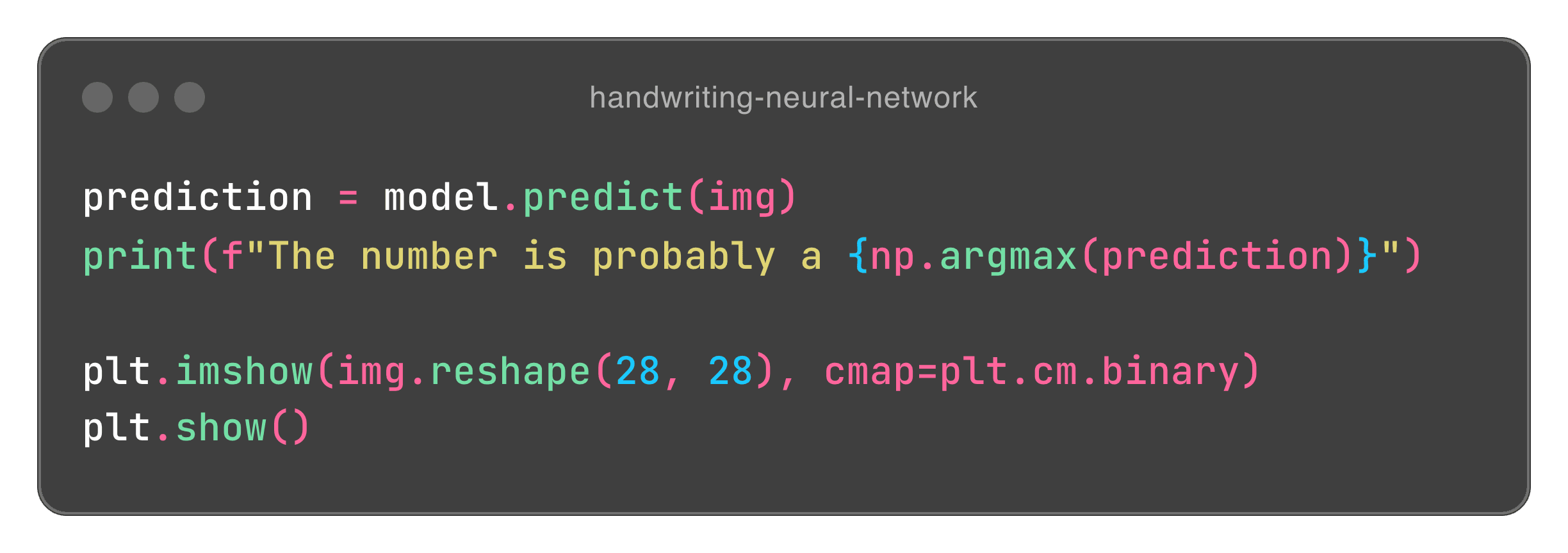
Here, we get the prediction of our model. It will provide us with an array of probabilities. For what our number could potentially be. Our np.argmax provides us with the maximum number, and returns that to the user. We then show the image in a 28 x 28 grid in binary (black and white) format, and show it to the user.

And thats it! When we run our main.py file, we get printed to the console:

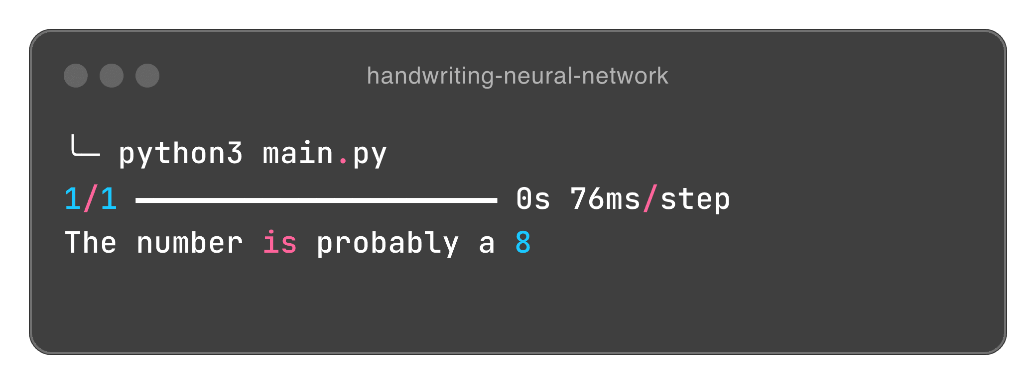
and the user is shown their image:

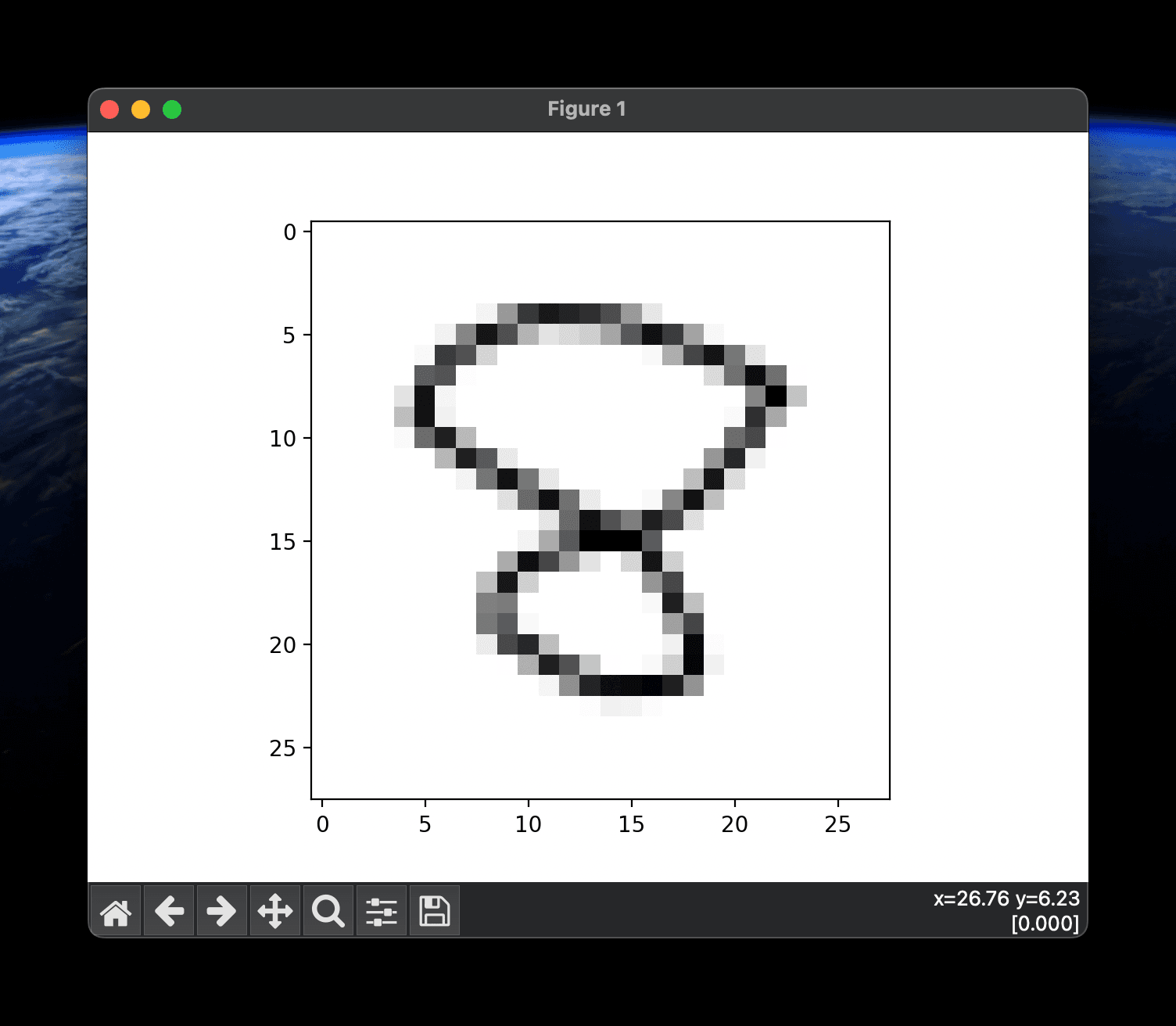
And there you have it! A neural network for recognising handwritten digits! There are some problems, such as if we upload the number 1 written on the far right, it may think its a four, but that’s because the MNIST dataset contains images that are all centred. A four has a stem on the far right, which may make it seem like a 4 was provided. Something like a Convoluted Neural Network would be better here.

Hello!!!

import React from 'react'
import { FaCog } from 'react-icons/fa'

function ReaderSettings() {
return (
<div